Electric Fields
Cornucopias of emission
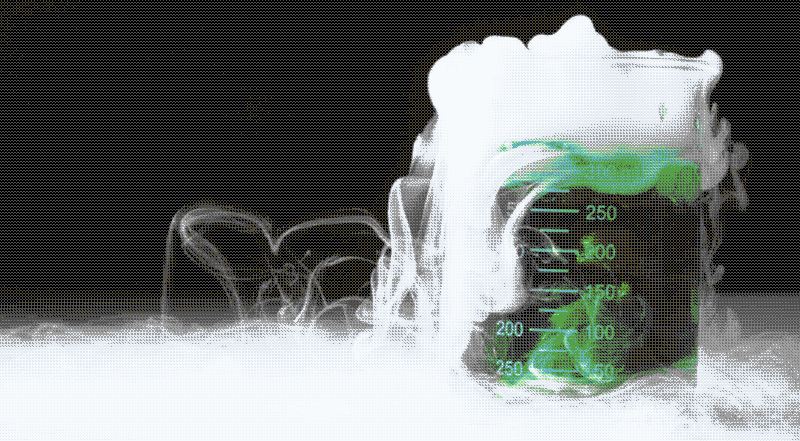
After we have established a set of pixels as our electrodes, we need to generate the electric fields. The specifics of how this is done is covered in more detail in the section on the Laplace equation. The way I think of these electric fields is that they are continuously emitted by each pixel, a bit like the smoke coming out of the beaker in the image above. The smoke spills over the edge and pools below the beaker, spreading out and dispersing. If the beaker were placed in a bowl, the smoke would eventually fill the bowl to the level of the beaker.
Now this analogy obviously has some problems. The smoke is highly chaotic and disperses over time. Electric fields are smooth and transition much more gently than the smoke. Even so, I think that this helps provide a better understanding of the nature of a static electric field: it is best to think of it as something that is static because it is being emitted, flowing, and then being “consumed” by electrodes all in an equilibrium, rather than something that is static because it is rigidly in place.
Thinking of electrodes in this way can help make clear the importance of choosing what goes on at the simulation boundary. When we get to one of the edges of our simulation, what should the “smoke” do? One option is to assume that the simulation is like a table, so the smoke will reach the edge and disappear off of it. Another option is to assume that the simulation is more like a table with a tall border around it, so when the smoke reaches the border, the overall level of smoke will begin to rise until it is all at the same level.
SIMION chooses the second approach, so the Simulation Playground does as well. You can verify this by erasing everything except one of the red circles in the example. Then define an electrode to be 0 Volts and put a pixel or two of it inside the red circle. You should see something like the image below after clicking

If you left the quadrupole electrode at 40 V, then when hovering your mouse around the dark red area, you can observe (using the cursor status readback) that the voltage at any area should be within a few tens of millivolts from 40 V. If this were solved analytically, everywhere outside of the circular red electrode would be exactly 40.0 V — the same as the value of the red electrode.
If, in contrast, you put a border of pixels around the whole electrode canvas and set this border to 0 V (the equivalent of removing the wall around the table in our analogy) or of putting the electrode in a grounded vacuum chamber, you should see a gradual tapering of the electric field from the red electrode to the outside:

The two views above help to show how fields refined from identical electrodes can exhibit very different behavior depending on the boundary conditions. Although SIMION and the Simulation Playground assume one behavior, it may be that a more accurate simulation requires the other boundary behavior. An obvious example is when the ion optics are inside of a grounded vacuum chamber. Vacuum chambers are almost always metal, and therefore they can lead to conditions more accurately modeled by the second example’s boundary conditions.