Heat equations

Finding the temperature of a rod

Hot metal forging photo by Tima Miroshnichenko from Pexels

In order to calculate the electric fields from our electrodes, we need to solve Laplace’s differential equation. 3Blue1Brown’s Grant Sanderson excellently describes differential equations and how much of the history of differential equations is wrapped up in calculating heat. For instance, Joseph Fourier famously described how heat flows along a rod and the Fourier series is integral to describing the temperature flow that occurs when a hot and cold rod meet.

Instead of two rods, we could imagine a flat sheet of metal that is heated (or cooled) continually at a point. We can think of this point like the contact of a water-heated metal pipe bent at 180°. As long as the hot water keeps flowing, the outside of this pipe will always be at a constant temperature. If we touch the bend of the pipe heated in this way to the metal plate, the plate will begin to heat at the contact point. The heat will be conducted away from the contact point and eventually the whole sheet of metal will be the same temperature as the heated pipe.

If we added a second bent pipe with cold water flowing through it, then after some time the sheet of metal would reach an equilibrium — with heat flowing from the hotter pipe, travelling through the metal sheet, and entering the cooler pipe. As long as the water in both pipes kept flowing at the same rate and at the same temperature, the temperature at any given point on the metal sheet wouldn’t change over time. If we visualized the temperature of the sheet using a heatmap, the result might look something like this:

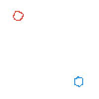
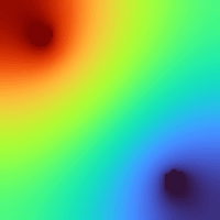
Where the left image shows the contact points of the hotter (red) and colder (blue) pipes and the right image shows the temperature at various points.

The plots above should be immediately familiar because they could just as easily represent electrodes with higher and lower voltages in a 2D plane. Laplace’s equation describes both static systems of heat as well as electric fields. Understanding that Laplace’s equation applies to heated systems as well as electric fields can help make one way of solving it, the finite difference method, a bit more intuitive.

Solving Laplace’s Equation

With The finite difference method

The finite difference method (FDM) solves Laplace’s equation numerically by iteratively “diffusing” the “heat” a little bit at a time. For each point of a 2D surface, the point is replaced by an average of the points above, below, left, and right — a configuration known as the five-point stencil. This can be observed numerically — I’ll round numbers to the nearest integer to keep everything tidy. We will start with a 5×5 grid of numbers and set the middle number to 100. This starting point with the 100 is special, as it is the “contact” point (for heat) or the “electrode” (for electric fields), so it will not change after each cycle.

As previously discussed the choice of boundary conditions matters here. Upon finding a boundary, we will calculate the values of the boundary points as the average of the adjacent points — so for the middle point on the top boundary, this is the points below, left, and right of it.

We could keep going forever, with each iteration getting closer to making all the numbers in the 5×5 closer to the original 100. Generally, we stop after hitting some metric that we decide is “good enough”. This might be a set number of iterations (say, 1 million iterations), a threshold for change between iterations (maybe 0.01 is a small enough change), or maybe we know the answer at a particular point and we stop when we get close enough.

Things might get a bit more interesting if we put two Dirichlet boundary condition values — say 100 and -70 — at opposite sides of the 5×5 grid. I will use a quick Python script to find the result after ten thousand iterations and then plot that as a heatmap:

And that’s it — we have solved Laplace’s equation for the 5×5 array with the boundary conditions. For all of the cells, taking the average of the above, below, left, and right cells (where possible) yields the current value of the cell (within 0.5 units as I rounded). This indicates that we have converged on a solution.

Earnshaw’s Theorem

How SIMION and the Playground get it wrong

One problem with this method of finding the electric field is that it is an approximation — one that we can make as accurate as we would like by trading more precision for longer refinement times. As the goals of SIMION are for accurate simulations, SIMION is generally accurate to at least to the millivolt. The Simulation Playground, that strives for speed and interactivity is not nearly as precise and may be wrong up to a few volts, especially when electrodes are set to many kilovolts. In most cases, these inaccuracies can be ignored. However, understanding how the electric fields are generated is useful to recognize the few cases where the inaccuracies do matter. One of the easiest inaccuracies to observe and test is that Earnshaw’s theorem is easily violated with both SIMION and the Simulation Playground.

Although there are many cases where we can see Earnshaw’s theorm hold true in SIMION and the Simulation Playground, it is very easy to construct a scenario with an electrostatic trap that causes ions to be statically trapped. One such example of Earnshaw’s therom falure is shown below, where an electrode ring of 20 kV is refined and then three ions are flown with a bit of random kinetic energy to demonstrate the “trap”. They yield stable orbits that would be impossible with a completely accurate simulation. The example shows their dynamic orbits intentionally, as observing statically-trapped ions would be relatively boring — they would just be a single, unmoving dot.

Small inaccuracies in the simulated fields can cause incorrect results.

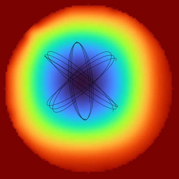
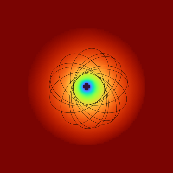
The reason why this simulation yields stable, static trajectories for many ions (i.e., violates Earnshaw’s theorem) is because of the way that the electric field was calculated. In actuality, the field within the ring would be exactly and homogenously 20 kV, so the ions would simply continue travelling in a straight line and impact the electrode. However, the simulation is not accurate — as we can easily observe the blue, lower-voltage center of the electric field. At its blue-colored center, the electric field was calculated to be 19,992 kV — eight volts less than the outside ring. This simulated inaccuracy is only 0.04%, but creates enough of a “bowl” shape that the ions cannot escape and are stably trapped.

Increasing the “field accuracy” parameter from “medium” to “highest” in the Simulation Playground’s Advanced tab can reduce this eight volt error down to 0.07 V (0.00035%), but refining takes quite a bit more computer power. To visualize this “bowl” shape, it may help to use the 3D viewer under the advanced tab. A similar inaccuracy, although much less pronounced, may be observed with SIMION in both 2D and 3D. For instance, instead of a circle, we could construct a large, hollow sphere in SIMION that would have the same low-voltage center, effectively trapping ions in similar violation of Earnshaw’s theorem.

Another inaccuracy in the electric fields is somewhat obvious and displeasing — the bowl is not even shaped nicely! The blue “dip” is off-center. This is due to the method of skipped point refining that is discussed in more detail in the page on Bonus details.

An electrostatic trap that can trap charged particles, in apparent violation of Earnshaw’s theorm, is the Kingdon trap. The Kingdon trap, and the more recent Orbitrap, trap ions dynamically. An example shows how this can be done:

Ions retain angular momentum in the Kingdon trap and are dynamically trapped

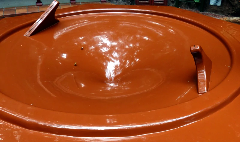
Ions in a Kingdon trap orbit an oppositely-charged central wire. The electrostatic potential shape is a bit like a hyperbolic cone or funnel, much like the spiral wishing wells, where a wisher would drop a coin down an inclined ramp, imparting an amount of angular momentum to their coin that would then race around in Spirograph-like patterns. Eventually friction would cause the orbit of the coin to decay, causing it to roll faster and faster around the center before dropping out of sight.

Coins roll around a funnel-shaped “spiral wishing well” by Unknown from Pikist

Ions, especially simulated ones, do not experience air or rolling friction and so do not decay as rapidly, however they will eventually lose energy — their angular momentum — due to image current effects and impact the central wire or spindle.