Simulations in five dimensions
Somebody get me a map
As could be observed in the previous section on visualization, the 2-dimensions of the electric fields can be viewed with a third dimension, voltage or potential either as a heatmap or as a heightmap (or both, in the case of the 3D view of the Simulation Playground). In reality, the simulation has a fourth dimension — time. As covered in the page on charged particles, at each timestep, we find the ion’s location, use it to get the electric vector, use that to get the forces on the ion and from those forces we get a cascade of acceleration, velocity, and finally position.
The code for this update runs in a “loop” — literally a “for” loop — until the ion has hit an electrode or the edge of the simulation, which ends the simulation and is called a “splat”. In the Simulation Playground, the simulation can also end after, a predetermined number of steps has passed, by default 400,000 steps, with each step being equivalent to a nanosecond.
          dt = 1E-9 # Conversion from seconds to nanoseconds
          position_log = []
          position = [initial_x_position, initial_y_position]
          for time in range(1, 400_001): # Keep going for 400,000 steps
              electric_vector = get_electric_vector(electric_field_map, position)
              force = charge * electric_vector
              acceleration = force / mass # Roll the golfball down the hill
              velocity += acceleration * dt
              position += velocity * dt
              position_log.append([position, time]) # Log position at each time
              if ion_has_splatted(position, electrode_map, boundaries):
                  print('SPLAT!')
                  break # We've hit something, stop the simulation
In the code above, the initial x and y coordinates are put into the “position” variable, which is then used, updated, logged, and then a conditional check (the function “ion_has_splatted”) checks if the position is outside the boundaries or within an electrode.
Hopefully you can see from the example code above that extending a simulation to another dimension — the z-axis — would only take a very minor update to the ion flight trajectory calculations. We would only need to add an “inital_z_position” variable and make sure that the “get_electric_vector” and “ion_has_splatted” functions worked in three dimensions! Similarly, we could extend it to a fourth (or fifth, or sixth, etc.) spatial dimension, just add a fourth “initial_w_position” variable and do the same checks.
Pixels versus voxels
Two out of three ain’t bad
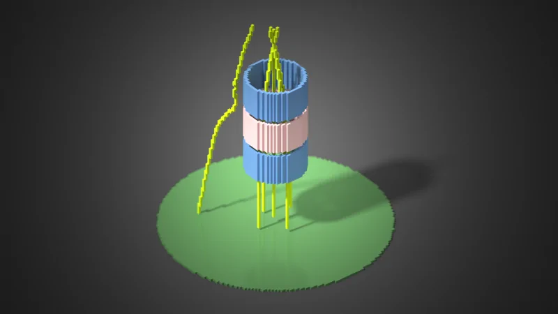
Although adding another spatial dimension has some major advantages — not least of which is that we live in 3-spatial-dimensions, it comes with two major disadvantages. First, those “grids” of 100 × 100 cells that I mentioned would then become cubes of 100 × 100 × 100 cells, from ten thousand to a million cells. One million is not a lot, in bytes it’s one megabyte, but the cube grows… well cubed. So if we wanted to simulate a 1 meter cube at a 250 micrometer resolution — which is still pretty coarse for “real life”, then at 1 byte per voxel we’d end up with a 64 gigabyte cube of voxels whereas an equivalent 2-dimensional grid of pixels would take 16 megabytes. In reality both numbers are bigger than this, but the square-cube relationship holds.
The second major disadvantage, and the one that led to the Simulation Playground staying in 2-dimensions, is that both creation and visualization of objects in three spatial dimensions is difficult to do and runs into some problems using current mouse-and-monitor-based computers.
The question then becomes, “how needed are three dimensions?” The answer, at least for professional instrument design, is that the costs are obviously worth the advantages. However, for simulation education and even early professional work, more can be done with two dimensions than you might expect. After all, SIMION started off as a 2-dimensional simulation program.1
The reason that two dimensions often suffices is that events in the ion-optical world often take place in a single plane. Ions with stable trajectories in the plane of interest are likely to have stable trajectories in all planes of a 3-dimensional view. Of course, this is not always the case — for example, there is no satisfactory way of fully simulating or depicting an Orbitrap mass analyzer in two dimensions.