Why simulations?

If we’re all living in one, let’s just go outside

Bubble chamber: color enhanced tracks, photo number CERN-EX-66954B by CERN

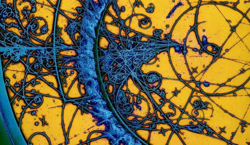
The image above shows tracks of charged particles, likely mesons that originate from a fast-moving neutrino in the Big European Bubble Chamber — decomissioned in 1984. The blue tracks we see were tiny bubbles that formed as fast-moving particles passed through a superheated mixture of liquid hydrogen and neon. A giant superconducting magnet produced a field that caused the charged particles to spiral. Five cameras mounted above the chamber quickly took photographs of the tracks for later analysis.

Today we have better methods of acquiring particle trajectory information, but the fact remains that it is hard to see ions and electrons move and it is nearly impossible to see their trajectories in a vacuum chamber. Charged particle optics shares much in common with light optics — including having interactive simulation websites. However, it is relatively easy to visualize, adjust, and experiment with light optics on an optical table. Although mostly used for toy demonstration purposes, smoke can even be blown over the optical table, causing light to scatter and be seen. No such visualization tricks are able to be performed in vacuum chambers.

Because of this, CAD software and simulations are usually the most efficient methods of designing and optimizing charged particle optics, at least in the inital phases. At this point, almost every electron gun, synchrotron, and mass spectrometer starts as a simulation.

Steps of a simulation

A brief overview

The four major steps of simulating ions are:

Both SIMION as well as the Simulation Playground follow these steps, although the specifics might be a bit different. For instance, there are only two ways of defining electrodes in the Playground: using a built-in simulation like the Lens simulation or by painting your own. SIMION has a few ways of defining electrodes, including importing them from another program, programmatic generation, GEM file creation, or using the builtin editor.

Pixels, Voxels, and Electrodes

1’s and 0’s pretending to be charged metal

We generate electrodes in the real world by shaping and then charging bits of metal. Mathematically representing these bits of metal and calculating the electric fields from them is routinely performed in the first year of physics. These calculations assume easy-to-define shapes such as perfect spheres, cubes, or planes. The solutions to these problems generally involve lots of equations and they provide exact, often mathematically beautiful, solutions. These type of problems are often solved with a pencil and paper. In mathematical language, this is called an analytical solution. Calculating electric fields and forces on ions analytically works well in rather simple cases but attempting to find an electrical field with more than a few electrodes or even a single electrode that is an irregular, asymmetrical shape can become very tedious or even impossible in practice.

Instead of perfect mathematical solutions, the way electric fields are generated in SIMION and the Simulation Playground is by approximation. Shapes are approximated as collections of pixels (in 2D) or voxels (in 3D). By approximating shapes as collections of rectangles or their 3D equivalents (called rectangular cuboids), electric fields can be estimated by repeated refinement steps that get closer to the solution with each step. This way of solving equations is known as numerical analysis. Newton’s method is one particularly well-known method of finding solutions of roots numerically.

In the Simulation Playground, all pixels that you draw to the screen are exactly square and represent fixed 2×2 mm blocks. The downside of this is that it limits the precision of an electrode. For instance, the Quadrupole simulation approximates 16 mm circles by pixelating them:

The builtin example for simulating a quadrupole in SIMION is a bit more accurate — it uses 23 pixels to simulate half of a circle (as the other half is redundant). So the quadrupoles in the SIMION example are better approximations than those in the Playground, but even these still have corners or roughness caused by the square pixels. Real quadrupoles don’t have any roughness — they are smooth rods that are precision machined to be circular or hyperbolic. More accurate approximations of these smooth edges could be made by making the pixels smaller and smaller. However, a smaller pixel size means that the number of calculations grows and the speed of simulating would decrease.

Although rough approximations of smooth shapes is inaccurate, it is fast both to simulate as well as to make with a simple pixel editor like the one included in the Simulation Playground. Internally, the pixel editor stores an array of pixels, not unlike a spreadsheet where each pixel is defined as an electrode. For instance, the pixelated circular quadrupole above is represented as an array of pixels where each pixel indicates which electrode it belongs to:

In this case, the “0” pixels belong to the white background and the blue “3” pixels indicate that this is the third, blue, electrode. If they were a “1” then they would be the first (red) electrode.